


台灣控制學習營: 平衡小車倒立單擺
Find AI Tools in second
Find AI Tools No difficulty
No complicated process
Find ai tools
No difficulty
No complicated process
Find ai tools


Table of Contents
Most people like

Flowtica AI,

 < 5K
< 5K
 100%
100%
 0
0
Your AI secretary - Todo, idea and meeting note, all flow with your voice.
AI Voice Assistants
Recording
AI Productivity Tools
AI Scheduling
Life Assistant
AI Meeting Assistant
AI Notes Assistant
AI Task Management
AD

Virbo AI Talking Photo
2.8M
 19.5%
0
19.5%
0
Create talking e-cards and portraits with AI.
AI Selfie & Portrait
Image to Video
Text to Video
AI Personalized Video Generator
Text-to-Speech
AI Speech Synthesis
AD
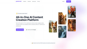
Postcrest
5.3K
18.88%
2
All-In-One AI Content Creation Platform for Social media
AI Productivity Tools
Speech-to-Text
Text to Video
AI UGC Video Generator
AI Video Generator
AI Short Clips Generator
AI Lip Sync Generator
Text-to-Speech
AI Voice Cloning
AI Face Swap Generator
AI Instagram Assistant
AI Twitter Assistant
AI YouTube Assistant
AI Facebook Assistant
AI Tiktok Assistant
AI Social Media Assistant
Digital Marketing Generator
Image to Video
AI Cosplay Generator
Text to Image
AI Photography
AI Selfie & Portrait
AI Photo & Image Generator
AI Avatar Generator
Image to Image
AI Background Remover
AI Profile Picture Generator
Photo & Image Editor
AI Photo Enhancer
AI Music Video Generator
AI Manga & Comic
AI Pattern Generator
AI Image Enhancer
AI Logo Generator
AI Cover Generator
AI Banner Generator
AI Background Generator
AI Illustration Generator
AI Content Generator
AD

MakeInfluencer AI
90.8K
 50.53%
4
50.53%
4
Create and monetize AI influencers for audience engagement.
AI Character
AI Social Media Assistant
AI Bio Generator
AI Content Generator
AI Avatar Generator
AI Profile Picture Generator
AI Chatbot
AI Instagram Assistant
AI Twitter Assistant
AI Facebook Assistant
AI Tiktok Assistant
AD
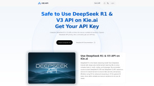
Kie.ai: Affordable & Secure DeepSeek R1 API
< 5K
1
Affordable DeepSeek R1 API with powerful reasoning and robust security.
AI Productivity Tools
AD
Are you spending too much time looking for ai tools?
- App rating
- 4.9
- AI Tools
- 100k+
- Trusted Users
- 5000+
 WHY YOU SHOULD CHOOSE TOOLIFY
TOOLIFY is the best ai tool source.
Browse More Content
Hardware-tw
- 英特爾酷睿i5 4430哈斯威爾處理器評測
- 100°C成為新常態!Intel Core i9-13900K對比i9-12900K以及Ryzen 9 7950X
- Intel 迫切需要另一款 2500K 處理器
- AMD Ryzen 6000、7000流言爆料!GTC回顧
- 2024年頂尖遊戲處理器推薦!
- Dell Precision 5530|SSD 1TB|RAM 32GB|I7 8850H|Quadro P1000|4K 15.6吋|像全新98%
- 超頻 AMD 1055T Phenom II X6
- 4萬台幣最佳筆記型電腦評估與比較
- AMD Ryzen 7800 X3D比Intel 13900K快25%!
- AMD 1055T 七年後仍能上遊戲嗎?
Related Articles


Refresh Articles
