


Mastering Regression Analysis: Understanding Slope and Y-Intercept
Find AI Tools No difficulty
No complicated process
Find ai tools
No difficulty
No complicated process
Find ai tools


Most people like
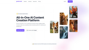
Postcrest

 5.3K
5.3K
 18.88%
 2
2
All-In-One AI Content Creation Platform for Social media
AI Productivity Tools
Speech-to-Text
Text to Video
AI UGC Video Generator
AI Video Generator
AI Short Clips Generator
AI Lip Sync Generator
Text-to-Speech
AI Voice Cloning
AI Face Swap Generator
AI Instagram Assistant
AI Twitter Assistant
AI YouTube Assistant
AI Facebook Assistant
AI Tiktok Assistant
AI Social Media Assistant
Digital Marketing Generator
Image to Video
AI Cosplay Generator
Text to Image
AI Photography
AI Selfie & Portrait
AI Photo & Image Generator
AI Avatar Generator
Image to Image
AI Background Remover
AI Profile Picture Generator
Photo & Image Editor
AI Photo Enhancer
AI Music Video Generator
AI Manga & Comic
AI Pattern Generator
AI Image Enhancer
AI Logo Generator
AI Cover Generator
AI Banner Generator
AI Background Generator
AI Illustration Generator
AI Content Generator
AD

MakeInfluencer AI
90.8K
 50.53%
4
50.53%
4
Create and monetize AI influencers for audience engagement.
AI Character
AI Social Media Assistant
AI Bio Generator
AI Content Generator
AI Avatar Generator
AI Profile Picture Generator
AI Chatbot
AI Instagram Assistant
AI Twitter Assistant
AI Facebook Assistant
AI Tiktok Assistant
AD
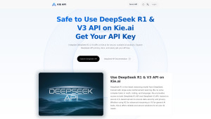
Kie.ai: Affordable & Secure DeepSeek R1 API
< 5K
1
Affordable DeepSeek R1 API with powerful reasoning and robust security.
AI Productivity Tools
AD
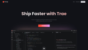
Trae
1M
 44.54%
1
44.54%
1
Adaptive AI IDE that helps you ship faster.
AI Code Generator
AD
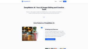
DeepMaker AI
< 5K
4
AI Image Editing Tools for Professionals
Text to Image
Photo & Image Editor
AI Tattoo Generator
AI Manga & Comic
AI Background Remover
AI Profile Picture Generator
AI Photo Restoration
AI Photo Enhancer
AI Logo Generator
AI Photo & Image Generator
AI Image Enhancer
AI Icon Generator
AI GIF Generator
AI Emoji Generator
AI Background Generator
AI Avatar Generator
AI Illustration Generator
AI Face Swap Generator
AD
Are you spending too much time looking for ai tools?
- App rating
- 4.9
- AI Tools
- 100k+
- Trusted Users
- 5000+
 WHY YOU SHOULD CHOOSE TOOLIFY
TOOLIFY is the best ai tool source.
Browse More Content
AI News
- Unveiling IA-Cloud: A Revolutionary Perspective by UiQ
- Unlocking the Power of Embedded AI Systems and Edge Computing
- Revolutionize Your Email Marketing with AI in 7 Steps
- Best Automated Crypto Trading Bots for Smarter and Profitable 24/7 Trading in 2023
- Best Website for Crypto Trading: Top Platforms for Beginners and Advanced Traders in 2023
- Where to Trade Cryptocurrency: Best Platforms for Beginners and Experienced Traders
- Top 7 Cheapest Crypto Trading Platforms for Low-Fee Trading in 2023
- Top 3 Low-Fee Crypto Trading Exchanges to Maximise Your Profits in 2023
- Best Leverage Trading Platforms for Crypto: Top Choices for Safe and Profitable Trading
- Best Futures Trading Platforms for Crypto in 2023: Top Choices for Beginners & Experts
Stable Video Diffusion
- Transform Your Images with Microsoft's BING and DALL-E 3
- Create Stunning Images with AI for Free!
- Unleash Your Creativity with Microsoft Bing AI Image Creator
- Create Unlimited AI Images for Free!
- Discover the Amazing Microsoft Bing Image Creator
- Create Stunning Images with Microsoft Image Creator
- AI Showdown: Stable Diffusion vs Dall E vs Bing Image Creator
- Create Stunning Images with Free Ai Text to Image Tool
- Unleashing Generative AI: Exploring Opportunities in QE&T
- Create a YouTube Channel with AI: ChatGPT, Bing Image Maker, Canva
Gemini AI
- Google's AI Demo Scandal Sparks Stock Plunge
- Unveiling the Yoga Master: the Life of Tirumalai Krishnamacharya
- Hilarious Encounter: Jimmy's Unforgettable Moment with Robert Irwin
- Google's Incredible Gemini Demo: Unveiling the Future
- Say Goodbye to Under Eye Dark Circles - Simple Makeup Tips
- Discover Your Magical Soul Mate in ASMR Cosplay Role Play
- Boost Kidney Health with these Top Foods
- OpenAI's GEMINI 1.0 Under Scrutiny
- Unveiling the Mind-Blowing Gemini Ultra!
- Shocking AI News: Google's Deception Exposed!
Hardware
- Exploring Minecraft 19.2: Performance, Settings, and Skyward Adventure
- Unleash the Power: Building a Gaming PC with Server Gear
- How to Setup Xbox Game Pass Cloud Gaming on Android TV
- Unlocking the Full Potential of AMD 1055T: Overclocking Adventure
- Performance Test: 4 Two-in-One Devices Compared
- Gaming on an Nvidia Quadro Card: Can It Deliver a Satisfying Experience?
- Intel's New Core i9-14900K: Faster than Core i9-13900K?
- Unleashing the Power: Ryzen 7 1700 vs 2700X Performance Comparison
- Essential Hardware and Software for Starting a Business
- Want to enhance your VR headset experience with AI? Here's how to do it!
Related Articles


Refresh Articles
